In Search of Entropy

Resource constrained embedded systems may lack a generic solution or support for true random number generation. Algorithmic pseudorandom number generators can be used in such cases combined with sources of unpredictable and asynchronous events to generate a seed value. In this post I explore a few entropy sources available in embedded systems which can be used to generate a seed value.

All sources described below are not new and they were explored in other articles available on the web. My goal is to get some practical experience and briefly explain why they can produce entropy. The sources are selected with the assumption that an embedded system has no ways of communication with environment, i.e., no user input or external interfaces which can provide interrupt events at random time. Cryptography is also out of scope as cryptography grade sources of entropy need much more careful characterisation. My case studies include much simpler application for random numbers such as device ID generation on systems where there are no unique HW identifiers, initial state generation for a game field or generation of some magic numbers.

Testing

Deciding what is “random enough” is not simple as the quality of random data depends both on quality of pseudorandom number generation (PRNG) algorithm and the quality of entropy source providing seed values for the algorithm. PRNGs are out of scope of this post and I will study entropy sources only. I will use autocorrelation function(ACF) as the first step for quick estimation of a source. ACF does not necessarily characterize an entropy source as acceptable or poor, but it can help to detect sources which yield correlated samples and thus are weak entropy sources. This test is done with a relatively small amount of samples and can help to save time during tests as the second step demands a lot of data to be collected for processing and it can take much time with some entropy sources which yield samples slowly. The second step is to use the NIST Entropy Source Testing tool for min-entropy¹ estimation as a characteristic value. This tool defines two tracks for entropy estimation: one for independent and identically distributed (IID) data and the other for non-IID data. The recommendation in the tool repository states that most entropy sources are non-IID, so I will follow this recommendation and use non-IID track.

STM32 Nucleo-F446RE development board was used for all tests described below and I chose it mostly for rich set of peripherals suitable for testing.

Analog Sources

Analog-to-Digital (ADC) converters are included in wide range of embedded systems. Higher precision ADCs can have a fair amount of noise in the lower-order bits, so an ADC can be used as an easily available source of entropy. There are several noise sources which contribute to the ADC’s output code.

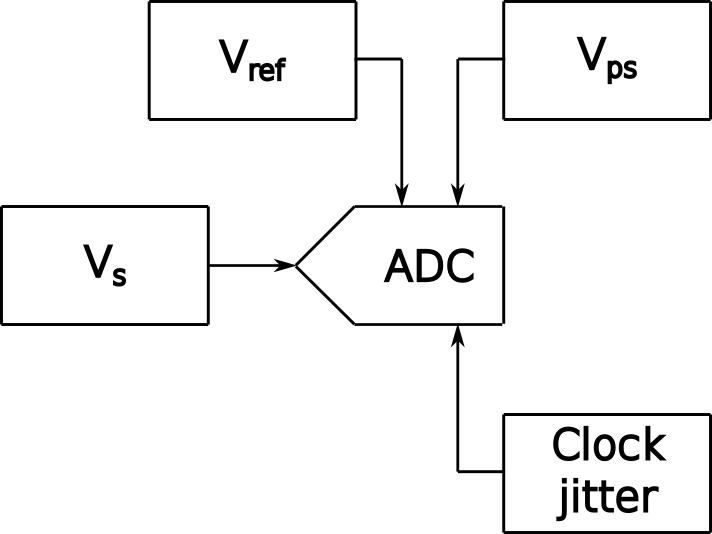
Vps and Vref are noise contribution from power supply chain and ADC’s reference voltage source. Vs is noise added from a sensor connected to the ADC and this component can contribute the most amount of noise in the system. Clock jitter translates to non-uniform signal sampling. Total internal ADC noise consists of two uncorrelated components: thermal noise and quantization noise. Quantization noise is a result of mapping of analog voltage which has infinite number of values to a digital code which has finite number of states. Thermal noise is inherent in all electrical components and for this reason it can be measured without applying an input signal. All these noise sources combined can produce a variation in the low-order bits of ADC’s output code.

To use ADC as an entropy source, it may be set to sample internal reference voltage or temperature sensor. Unconnected input pin should work too as it can be an equivalent of a poor antenna and inject noise from surrounding electromagnetic waves. If possible, it is better to set highest ADC resolution to maximise thermal noise over quantisation noise. Then read several samples and use only lower-order bit (or a few bits in case the input noise signal is high) to assemble a random byte. This procedure can be repeated to produce as many random bytes as needed. I used such procedure to collect one byte samples from internal temperature sensor and one unconnected GPIO configured as analog input. Samples were sent over UART to PC for storing and analyses. A data set of 100k samples was collected for the preliminary estimation.

Lets look at the ACF of the samples I collected.

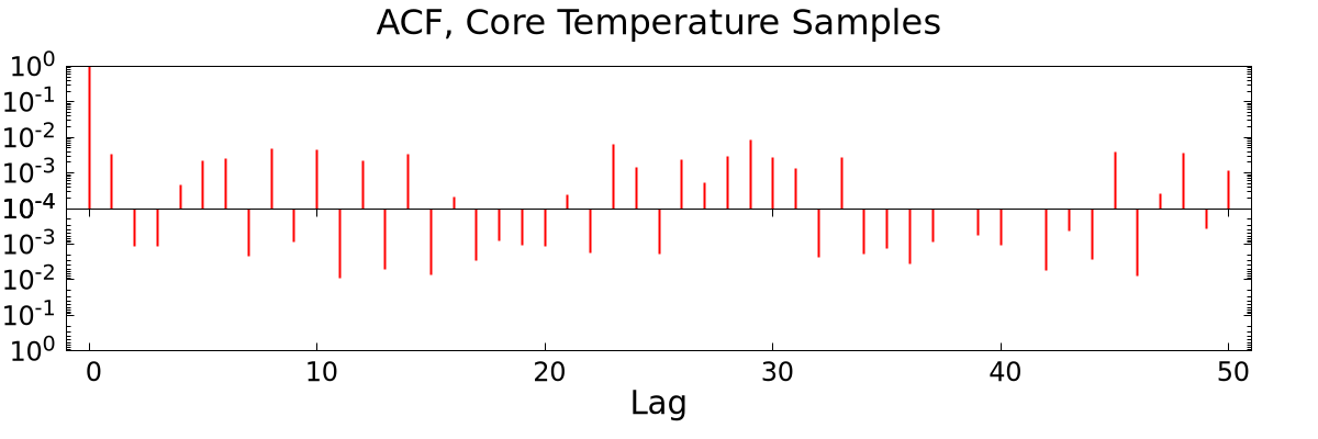
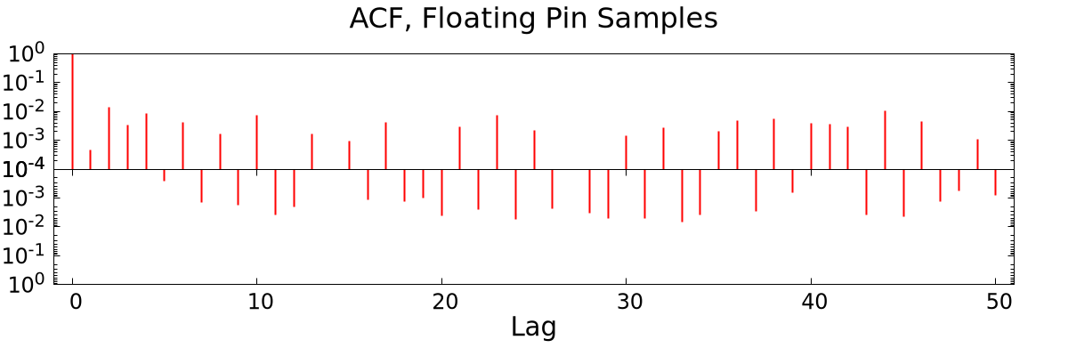
Both figures have logarithmic scale on y axis. The ACF in both cases is lower than 0.01 which suggests that the samples from both sources are not correlated and it is worth to analyse them further using time consuming methods. The lag on the figures is only 50 samples, but I also analyzed longer sample series to find possible long term periodicity. The ACF of the samples from floating GPIO pin shows some periodic structure in case much longer data set is analyzed. My guess is that it reveals the interference from power grid, but proving this is outside of the study.

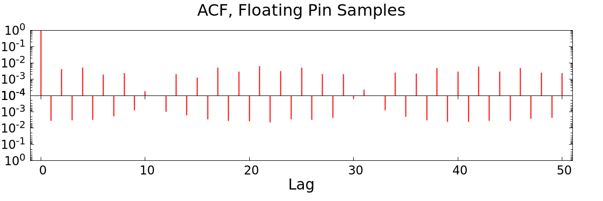
The next step would be to record 10 MB of samples from each source and feed them to the entropy assessment tool. I recorded several such sample files to calculate mean value of entropy over the collection. The core temperature samples produced 5.8 bits of entropy and the floating pin samples produced 6.0 bits of entropy.

Just out of curiosity, I also fed the stream of random bytes to dieharder test suite which is a collection of tests for random number generators. This test suite has various tests for estimating different aspects of random number generators, but I decided to use just one of them, STS Monobit Test, which is simple but effective at revealing overtly weak generators. Here s the result:

#=============================================================================#
#            dieharder version 3.31.1 Copyright 2003 Robert G. Brown          #
#=============================================================================#
   rng_name    |rands/second|   Seed   |
stdin_input_raw|  2.34e+03  | 691519662|
#=============================================================================#
        test_name   |ntup| tsamples |psamples|  p-value |Assessment
#=============================================================================#
         sts_monobit|   1|    100000|     100|0.00000000|  FAILED

The result clearly shows that this is a pretty weak random number generator.

SRAM Boot State

Here is a simplified schematic of a SRAM cell which stores one bit. The four transistors form two cross-coupled inverters which can be in two stable states.

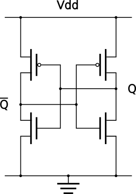
Power is applied to both inverters simultaneously at boot time and initially they are in a metastable state. Due to imperfections in manufacturing process, thermal noise and surrounding current flows one of the inverters will eventually become closer to its stable state and the cell will switch to 0 or 1. Most of the cells have not so well balanced transistors, so they always switch to the same state after power up. But a smaller part of the cells with highly symmetric inverters randomly switch to a stable state under random fluctuations of current flows. Such unstable SRAM cells can be used to harvest entropy.

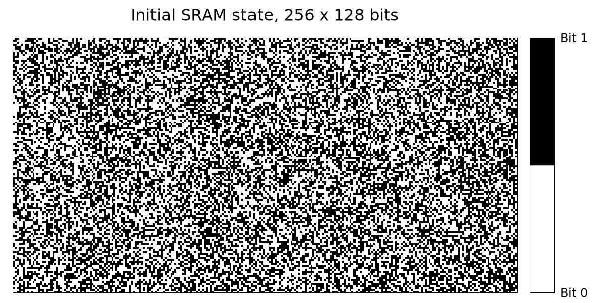
The following picture represents the initial SRAM state on my dev. board after power up and before it was initialized. This is only a small slice of SRAM for demonstration purposes and the pattern will be different for another MCU of the same type.

And here is a picture representing the difference between two SRAM states after a power cycle. White and grey pixels represent bits that have not changed after power cycle, blue pixels are bits that changed from 1 to 0 and red pixels are bits that changed from 0 to 1.

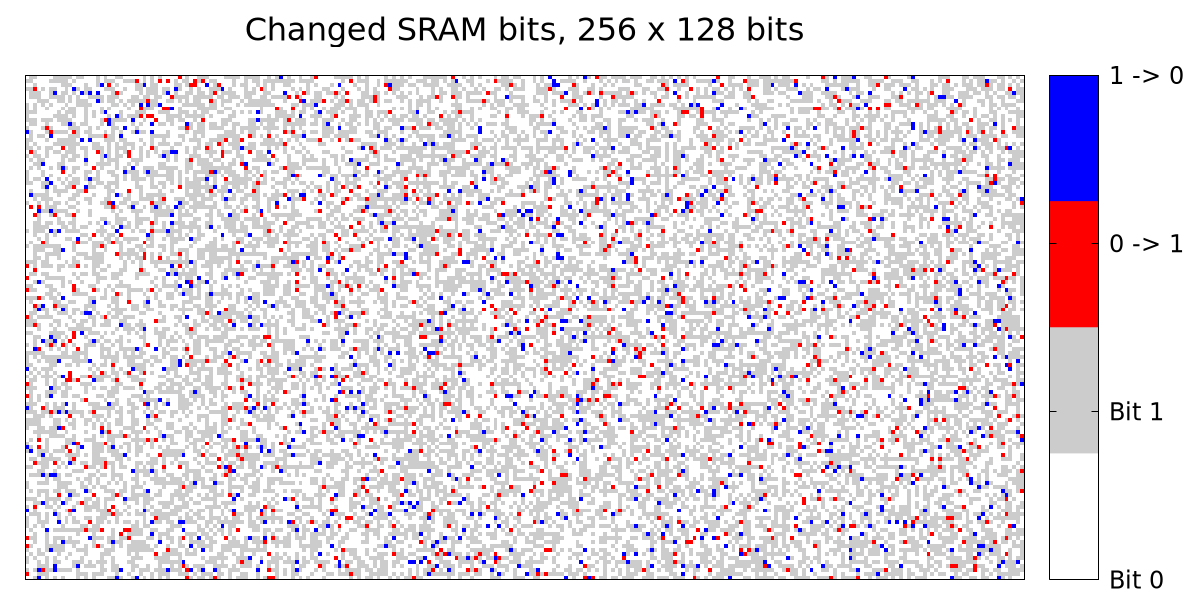
Clearly not many of them can switch randomly and yield entropy. I split total SRAM contents into 31 blocks each 4096 bytes in size and calculated the number of changing bits in each block. The mean value of changed bits was 2105.4 with standard deviation of 65.7 bits which means that there are no obvious differences between the blocks and that changing bits are spread more or less evenly across SRAM. Overall only 6.3% of bits changed their state after power cycle and the number is aligned with other sources describing the same experiment that I found on the web.

The idea of collecting entropy from SRAM state is simple: partition SRAM into blocks, XOR all bytes in the block to get one byte of entropy and repeat the procedure across all blocks. The number of blocks can vary depending on the number of bytes required at system start. I partitioned SRAM into 31 blocks of 4096 bytes for collecting data for the test. The MCU has more RAM available, but I excluded a few kilobytes in the beginning and the end of RAM space as they contain initialized data for running test program. This gave me only 31 bytes of data at each boot cycle and I needed to repeatedly reboot the MCU to collect the amount of data required for analyses. The MCU can not be just rebooted from software as such reboot does not power off the SRAM and its contents remain the same including uninitialised blocks. A cold reboot is needed for the purpose of the test. Rebooting the dev. board manually was not an option as it would require too much time to collect the amount of data necessary for the entropy estimation. Fortunately, the MCU supports a standby mode in which most of its peripherals including SRAM are turned off and I used this mode in a loop to generate a stream of random bytes. Test program just read the SRAM contents, transferred the data to a PC, set a watchdog timer and went into standby mode to have its SRAM contents erased. The watchdog timer is one of the few peripheral blocks which stays powered in standby mode so that it could reboot the MCU after timer expiration. The process repeated after MCU reboot to generate as much test data as needed.

While experimenting with the standby mode, I noticed that the overall number of changing bits depends on the time the MCU spent in the standby mode although the difference is not very high.

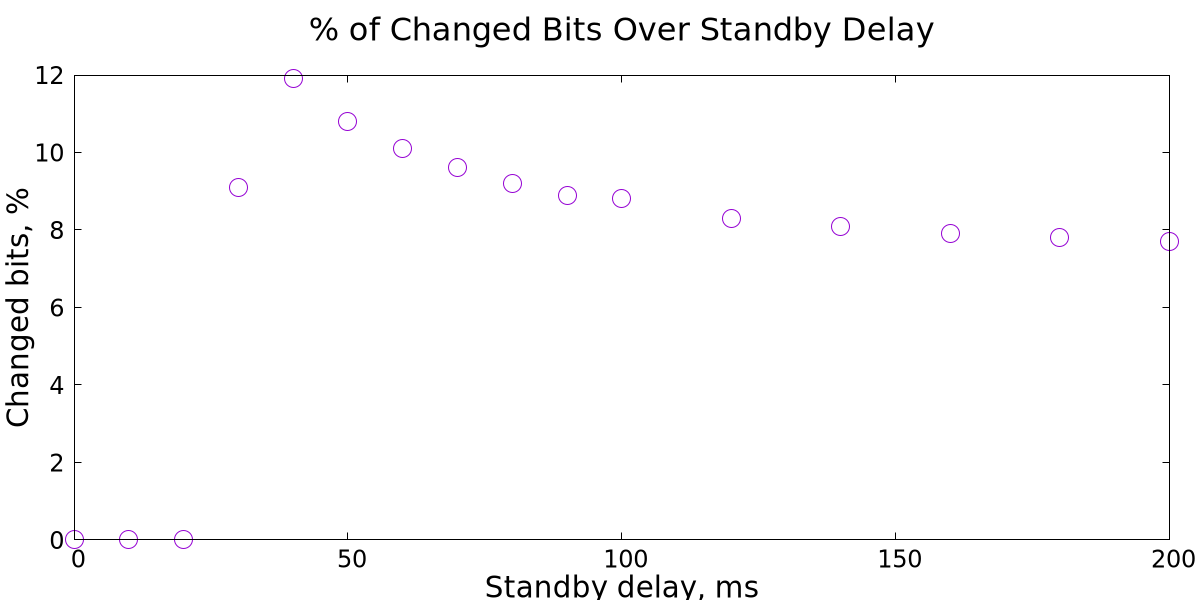
This could be explained by residual charges in the system after it was powered off. It takes some time for the system to fully discharge and if the SRAM is powered again soon enough, it can keep its contents unerased. In my case, standby mode duration of up to 20 ms did not change the SRAM contents and only 100 ms duration could give more or less stable results. The peak at 40 ms duration is probably the state where residual charges push more cells into a metastable state and more bits can switch their state during test cycle.

I decided to use 100 ms standby mode duration for further testing. As only 31 blocks of SRAM were used to produce one byte of random data per block, approximately 310 bytes per second yield ratio was expected from this method of entropy generation. This is where an ACF can be helpful as a preliminary analyses tool to decide if it is worth continuing the experiment. I collected 100k of samples and the results were promising.

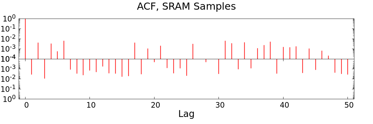
As with ADC sources, this method did not show any correlation between samples, so the experiment was continued for several hours needed to collect a full 10 MB data set for entropy estimation. I also repeated the experiment with 40 ms standby duration to check if it could give a better entropy value. Both experiments produced around 7.5 bits of entropy. It is hard to make conclusions based on a single experiment, but it would be safe to assume that both standby durations can produce comparable amount of entropy and from practical perspective it is better to use shorter duration.

Timing Various Processes

Some peripheral blocks in embedded systems can have nondeterministic startup time. Such blocks should have typical and maximal time specified in their documentation and the difference between the two can be significant. In most cases the difference is determined by temperature, power supply variations and different startup conditions specific to a peripheral block, but I was more interested in possible small run to run variations in stable conditions when the surrounding temperature and power supply remain unchanged. The idea was to check if such variations have stochastic nature and could be used as entropy source. The peripheral blocks which can be used for such test include RC oscillators, PLLs and external crystal oscillators. I decided to experiment with low-speed internal RC oscillator (LSI) and see if various types of noise inherently present in the system can influence its startup time.

The MCU documentation defines typical and maximal LSI startup time equal to 15 and 40 µs respectively. The absolute value does not matter as I was interested in run to run variation, so testing method in this case was almost the same as for ADC. The LSI was started and the program polled a status flag to wait for the LSI to be ready. The startup process time was measured with CPU cycles counter as the fastest counter running in the system. Also the CPU was running at maximal speed to increase the resolution of the measurement. Once the startup time was measured, only its least significant bit was used and then the LSI was stopped. This procedure repeated to produces as many bits as needed.

As in previous cases, initially I estimated the ACF of a 100k data set as bits generation rate was low and it could take some time to collect a full 10 MB data set.

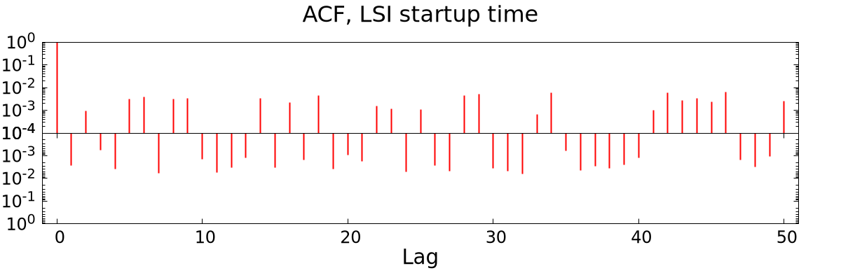
And again it was good enough to proceed with further collection and analysis. The entropy analysis tool calculated 7.5 bits of entropy in this experiment.

Another experiment with timing processes I made was measuring flash word programming and sector erase times. The MCU documentation states that the typical and maximal word programming times are 16 and 100 µs respectively. As for sector erase time, this value varies with sector size and erase parallelism. I chose 128 KB sector for the experiment and erase parallelism was set to x32. This particular sector was never used on this MCU before, so it could be considered new and without any wearing. The typical and maximal erase time in this case are 1 and 2 seconds respectively. The variation in programming and erase times is mostly related to flash wearing during its course of operation and it should not change significantly in the specified range from run to run. In my case the maximal erase time is characterized by manufacturer after 100k erase operations. But I was hoping to measure small variations in programming and erase time which can be used as a source of entropy. It tuned out that there are such time variations, so I continued with the experiment.

Entropy harvesting was made in the way similar to analog sources: measure processing time and use least significant bit as the most noisy one to assemble a byte. I used just one 128 KB flash sector for this experiment. It was sequentially programmed with random data and programming time of each 32 bit data word was measured. When the sector was fully programmed, I erased it and measured erase time as well, but this measurement was processed separately and was not mixed with programming time. This process was repeated as many times as was needed to collect a full 10 MB data set for entropy analyses. When the first 100k of samples were ready, I estimated the ACF to decide if it was worth to continue the experiment.

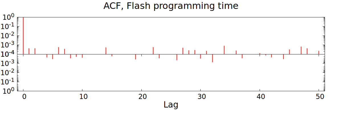
The correlation between samples in this case was even smaller than in all previous cases, although not much smaller. The total amount of entropy in this experiment was 7.4 bits.

Only few thousands of erase cycles were required to collect full data set based on word programming time and the MCU has only 10000 erase cycles guaranteed by the manufacturer. For these reasons it was not possible to collect a required amount of data for analyses based exclusively on erase time given that I used only one flash sector on a single MCU sample. Anyway I collected sector erase time during the experiment to see if this type of data could also be used for entropy harvesting.

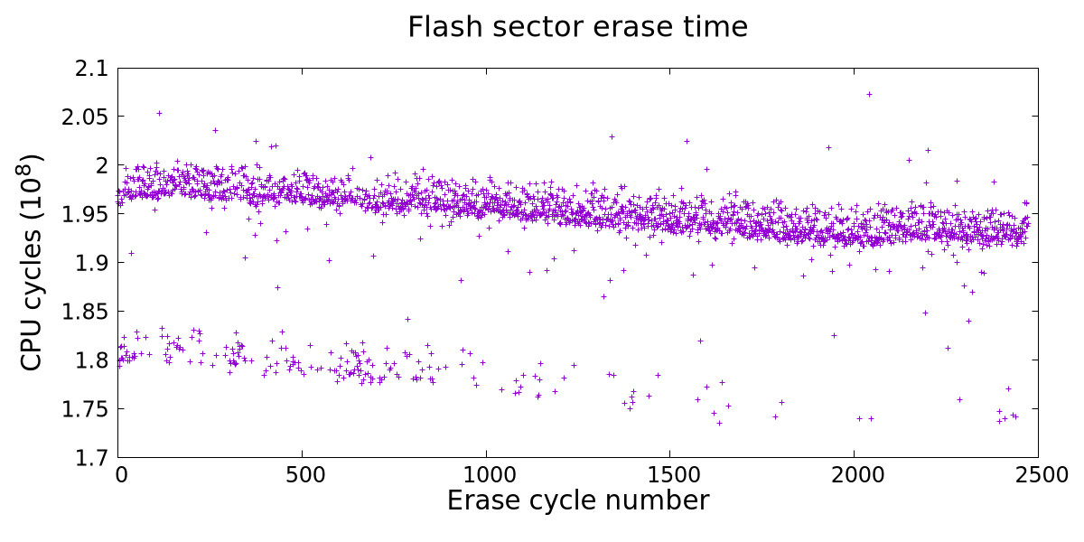
Sector erase time too has small variations which can possibly be used to harvest entropy, but more interestingly it demonstrated a bimodal distribution with lesser mode becoming less frequent over time which I did not expect. Modern flash chips can implement incremental erasure algorithms² which can have variable erasure time to minimize flash wearing and improve its lifetime, but I am not sure if something like this was implemented in a more than 10 years old MCU (STM32F446 production started in 2015). I don’t have a good explanation at the moment.

Save Entropy Across Reboots

A seed value can be generated on another system and stored on a target embedded system in case there are no entropy sources available in the system. The stored value can be used immediately after boot in this case. It makes sense to mix it with any fresh entropy which may be available during system operation at later time and store the new value for the next boot cycle. This method requires some flash memory for storage, but it should be available in most cases.

Conclusion

It is important to keep in mind that all methods described here are not suitable on their own for cryptography grade random numbers generation and such methods require careful characterization to prove reliability. In general they demonstrated good entropy levels for less demanding applications.

All these methods have their own strong and weak sides. ADC can produce infinite stream of random bits and do it fast, but it may not be available for this purpose because it is connected to external circuitry or not present in the system. SRAM boot state is the fastest method, but it has limited capacity and not suitable in case the system is always powered by battery and can not erase its data. Timing peripheral blocks startup may also have limited use and slow yield, but more importantly it requires high precision timer. Flash have limited endurance and not suitable as primary source for this reason. But all these methods can be combined in different variations to contribute to an entropy pool.